hypothesis regression analysis

Prompt Library
DS/AI Trends
Stats Tools
Interview Questions
Generative AI
Machine Learning
Deep Learning

Linear regression hypothesis testing: Concepts, Examples

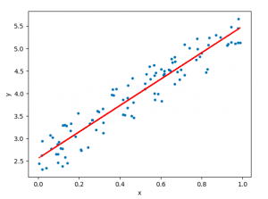
In relation to machine learning , linear regression is defined as a predictive modeling technique that allows us to build a model which can help predict continuous response variables as a function of a linear combination of explanatory or predictor variables. While training linear regression models, we need to rely on hypothesis testing in relation to determining the relationship between the response and predictor variables. In the case of the linear regression model, two types of hypothesis testing are done. They are T-tests and F-tests . In other words, there are two types of statistics that are used to assess whether linear regression models exist representing response and predictor variables. They are t-statistics and f-statistics. As data scientists , it is of utmost importance to determine if linear regression is the correct choice of model for our particular problem and this can be done by performing hypothesis testing related to linear regression response and predictor variables. Many times, it is found that these concepts are not very clear with a lot many data scientists. In this blog post, we will discuss linear regression and hypothesis testing related to t-statistics and f-statistics . We will also provide an example to help illustrate how these concepts work.

Table of Contents

What are linear regression models?

A linear regression model can be defined as the function approximation that represents a continuous response variable as a function of one or more predictor variables. While building a linear regression model, the goal is to identify a linear equation that best predicts or models the relationship between the response or dependent variable and one or more predictor or independent variables.

There are two different kinds of linear regression models. They are as follows:

Simple or Univariate linear regression models : These are linear regression models that are used to build a linear relationship between one response or dependent variable and one predictor or independent variable. The form of the equation that represents a simple linear regression model is Y=mX+b, where m is the coefficients of the predictor variable and b is bias. When considering the linear regression line, m represents the slope and b represents the intercept.
Multiple or Multi-variate linear regression models : These are linear regression models that are used to build a linear relationship between one response or dependent variable and more than one predictor or independent variable. The form of the equation that represents a multiple linear regression model is Y=b0+b1X1+ b2X2 + … + bnXn, where bi represents the coefficients of the ith predictor variable. In this type of linear regression model, each predictor variable has its own coefficient that is used to calculate the predicted value of the response variable.

While training linear regression models, the requirement is to determine the coefficients which can result in the best-fitted linear regression line. The learning algorithm used to find the most appropriate coefficients is known as least squares regression . In the least-squares regression method, the coefficients are calculated using the least-squares error function. The main objective of this method is to minimize or reduce the sum of squared residuals between actual and predicted response values. The sum of squared residuals is also called the residual sum of squares (RSS). The outcome of executing the least-squares regression method is coefficients that minimize the linear regression cost function .

The residual e of the ith observation is represented as the following where [latex]Y_i[/latex] is the ith observation and [latex]\hat{Y_i}[/latex] is the prediction for ith observation or the value of response variable for ith observation.

[latex]e_i = Y_i – \hat{Y_i}[/latex]

The residual sum of squares can be represented as the following:

[latex]RSS = e_1^2 + e_2^2 + e_3^2 + … + e_n^2[/latex]

The least-squares method represents the algorithm that minimizes the above term, RSS.

Once the coefficients are determined, can it be claimed that these coefficients are the most appropriate ones for linear regression? The answer is no. After all, the coefficients are only the estimates and thus, there will be standard errors associated with each of the coefficients. Recall that the standard error is used to calculate the confidence interval in which the mean value of the population parameter would exist. In other words, it represents the error of estimating a population parameter based on the sample data. The value of the standard error is calculated as the standard deviation of the sample divided by the square root of the sample size. The formula below represents the standard error of a mean.

[latex]SE(\mu) = \frac{\sigma}{\sqrt(N)}[/latex]

Thus, without analyzing aspects such as the standard error associated with the coefficients, it cannot be claimed that the linear regression coefficients are the most suitable ones without performing hypothesis testing. This is where hypothesis testing is needed . Before we get into why we need hypothesis testing with the linear regression model, let’s briefly learn about what is hypothesis testing?

Train a Multiple Linear Regression Model using R

Before getting into understanding the hypothesis testing concepts in relation to the linear regression model, let’s train a multi-variate or multiple linear regression model and print the summary output of the model which will be referred to, in the next section.

The data used for creating a multi-linear regression model is BostonHousing which can be loaded in RStudioby installing mlbench package. The code is shown below:

install.packages(“mlbench”) library(mlbench) data(“BostonHousing”)

Once the data is loaded, the code shown below can be used to create the linear regression model.

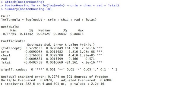
attach(BostonHousing) BostonHousing.lm <- lm(log(medv) ~ crim + chas + rad + lstat) summary(BostonHousing.lm)

Executing the above command will result in the creation of a linear regression model with the response variable as medv and predictor variables as crim, chas, rad, and lstat. The following represents the details related to the response and predictor variables:

log(medv) : Log of the median value of owner-occupied homes in USD 1000’s
crim : Per capita crime rate by town
chas : Charles River dummy variable (= 1 if tract bounds river; 0 otherwise)
rad : Index of accessibility to radial highways
lstat : Percentage of the lower status of the population

The following will be the output of the summary command that prints the details relating to the model including hypothesis testing details for coefficients (t-statistics) and the model as a whole (f-statistics)

linear regression model summary table r.png

Hypothesis tests & Linear Regression Models

Hypothesis tests are the statistical procedure that is used to test a claim or assumption about the underlying distribution of a population based on the sample data. Here are key steps of doing hypothesis tests with linear regression models:

Hypothesis formulation for T-tests: In the case of linear regression, the claim is made that there exists a relationship between response and predictor variables, and the claim is represented using the non-zero value of coefficients of predictor variables in the linear equation or regression model. This is formulated as an alternate hypothesis. Thus, the null hypothesis is set that there is no relationship between response and the predictor variables . Hence, the coefficients related to each of the predictor variables is equal to zero (0). So, if the linear regression model is Y = a0 + a1x1 + a2x2 + a3x3, then the null hypothesis for each test states that a1 = 0, a2 = 0, a3 = 0 etc. For all the predictor variables, individual hypothesis testing is done to determine whether the relationship between response and that particular predictor variable is statistically significant based on the sample data used for training the model. Thus, if there are, say, 5 features, there will be five hypothesis tests and each will have an associated null and alternate hypothesis.
Hypothesis formulation for F-test : In addition, there is a hypothesis test done around the claim that there is a linear regression model representing the response variable and all the predictor variables. The null hypothesis is that the linear regression model does not exist . This essentially means that the value of all the coefficients is equal to zero. So, if the linear regression model is Y = a0 + a1x1 + a2x2 + a3x3, then the null hypothesis states that a1 = a2 = a3 = 0.
F-statistics for testing hypothesis for linear regression model : F-test is used to test the null hypothesis that a linear regression model does not exist, representing the relationship between the response variable y and the predictor variables x1, x2, x3, x4 and x5. The null hypothesis can also be represented as x1 = x2 = x3 = x4 = x5 = 0. F-statistics is calculated as a function of sum of squares residuals for restricted regression (representing linear regression model with only intercept or bias and all the values of coefficients as zero) and sum of squares residuals for unrestricted regression (representing linear regression model). In the above diagram, note the value of f-statistics as 15.66 against the degrees of freedom as 5 and 194.
Evaluate t-statistics against the critical value/region : After calculating the value of t-statistics for each coefficient, it is now time to make a decision about whether to accept or reject the null hypothesis. In order for this decision to be made, one needs to set a significance level, which is also known as the alpha level. The significance level of 0.05 is usually set for rejecting the null hypothesis or otherwise. If the value of t-statistics fall in the critical region, the null hypothesis is rejected. Or, if the p-value comes out to be less than 0.05, the null hypothesis is rejected.
Evaluate f-statistics against the critical value/region : The value of F-statistics and the p-value is evaluated for testing the null hypothesis that the linear regression model representing response and predictor variables does not exist. If the value of f-statistics is more than the critical value at the level of significance as 0.05, the null hypothesis is rejected. This means that the linear model exists with at least one valid coefficients.
Draw conclusions : The final step of hypothesis testing is to draw a conclusion by interpreting the results in terms of the original claim or hypothesis. If the null hypothesis of one or more predictor variables is rejected, it represents the fact that the relationship between the response and the predictor variable is not statistically significant based on the evidence or the sample data we used for training the model. Similarly, if the f-statistics value lies in the critical region and the value of the p-value is less than the alpha value usually set as 0.05, one can say that there exists a linear regression model.

Why hypothesis tests for linear regression models?

The reasons why we need to do hypothesis tests in case of a linear regression model are following:

By creating the model, we are establishing a new truth (claims) about the relationship between response or dependent variable with one or more predictor or independent variables. In order to justify the truth, there are needed one or more tests. These tests can be termed as an act of testing the claim (or new truth) or in other words, hypothesis tests.
One kind of test is required to test the relationship between response and each of the predictor variables (hence, T-tests)
Another kind of test is required to test the linear regression model representation as a whole. This is called F-test.

While training linear regression models, hypothesis testing is done to determine whether the relationship between the response and each of the predictor variables is statistically significant or otherwise. The coefficients related to each of the predictor variables is determined. Then, individual hypothesis tests are done to determine whether the relationship between response and that particular predictor variable is statistically significant based on the sample data used for training the model. If at least one of the null hypotheses is rejected, it represents the fact that there exists no relationship between response and that particular predictor variable. T-statistics is used for performing the hypothesis testing because the standard deviation of the sampling distribution is unknown. The value of t-statistics is compared with the critical value from the t-distribution table in order to make a decision about whether to accept or reject the null hypothesis regarding the relationship between the response and predictor variables. If the value falls in the critical region, then the null hypothesis is rejected which means that there is no relationship between response and that predictor variable. In addition to T-tests, F-test is performed to test the null hypothesis that the linear regression model does not exist and that the value of all the coefficients is zero (0). Learn more about the linear regression and t-test in this blog – Linear regression t-test: formula, example .

Ajitesh Kumar

One response.

Very informative

Search for:

ChatGPT Prompts (250+)

Generate Design Ideas for App
Expand Feature Set of App
Create a User Journey Map for App
Generate Visual Design Ideas for App
Generate a List of Competitors for App
Agentic Reasoning Design Patterns in AI: Examples
LLMs for Adaptive Learning & Personalized Education
Sparse Mixture of Experts (MoE) Models: Examples
Anxiety Disorder Detection & Machine Learning Techniques
Confounder Features & Machine Learning Models: Examples

Data Science / AI Trends

• Sentiment Analysis Real World Examples
• Prepend any arxiv.org link with talk2 to load the paper into a responsive chat application
• Custom LLM and AI Agents (RAG) On Structured + Unstructured Data - AI Brain For Your Organization
• Guides, papers, lecture, notebooks and resources for prompt engineering
• Common tricks to make LLMs efficient and stable

Free Online Tools

Create Scatter Plots Online for your Excel Data
Histogram / Frequency Distribution Creation Tool
Online Pie Chart Maker Tool
Z-test vs T-test Decision Tool
Independent samples t-test calculator

Hypothesis Testing in Regression Analysis

Hypothesis testing is used to confirm if the estimated regression coefficients bear any statistical significance. Either the confidence interval approach or the t-test approach can be used in hypothesis testing. In this section, we will explore the t-test approach.

The t-test Approach

The following are the steps followed in the performance of the t-test:

Set the significance level for the test.
Formulate the null and the alternative hypotheses.

$$t=\frac{\widehat{b_1}-b_1}{s_{\widehat{b_1}}}$$

$b_1$ = True slope coefficient.

$\widehat{b_1}$ = Point estimate for $b_1$

$b_1 s_{\widehat{b_1\ }}$ = Standard error of the regression coefficient.

Compare the absolute value of the t-statistic to the critical t-value (t_c). Reject the null hypothesis if the absolute value of the t-statistic is greater than the critical t-value i.e., $t\ >\ +\ t_{critical}\ or\ t\ <\ –t_{\text{critical}}$.

Example: Hypothesis Testing of the Significance of Regression Coefficients

An analyst generates the following output from the regression analysis of inflation on unemployment:

$$\small{\begin{array}{llll}\hline{}& \textbf{Regression Statistics} &{}&{}\\ \hline{}& \text{Multiple R} & 0.8766 &{} \\ {}& \text{R Square} & 0.7684 &{} \\ {}& \text{Adjusted R Square} & 0.7394 & {}\\ {}& \text{Standard Error} & 0.0063 &{}\\ {}& \text{Observations} & 10 &{}\\ \hline {}& & & \\ \hline{} & \textbf{Coefficients} & \textbf{Standard Error} & \textbf{t-Stat}\\ \hline \text{Intercept} & 0.0710 & 0.0094 & 7.5160 \\\text{Forecast (Slope)} & -0.9041 & 0.1755 & -5.1516\\ \hline\end{array}}$$

At the 5% significant level, test the null hypothesis that the slope coefficient is significantly different from one, that is,

$$ H_{0}: b_{1} = 1\ vs. \ H_{a}: b_{1}≠1 $$

The calculated t-statistic, $\text{t}=\frac{\widehat{b_{1}}-b_1}{\widehat{S_{b_{1}}}}$ is equal to:

$$\begin{align*}\text{t}& = \frac{-0.9041-1}{0.1755}\\& = -10.85\end{align*}$$

The critical two-tail t-values from the table with $n-2=8$ degrees of freedom are:

$$\text{t}_{c}=±2.306$$

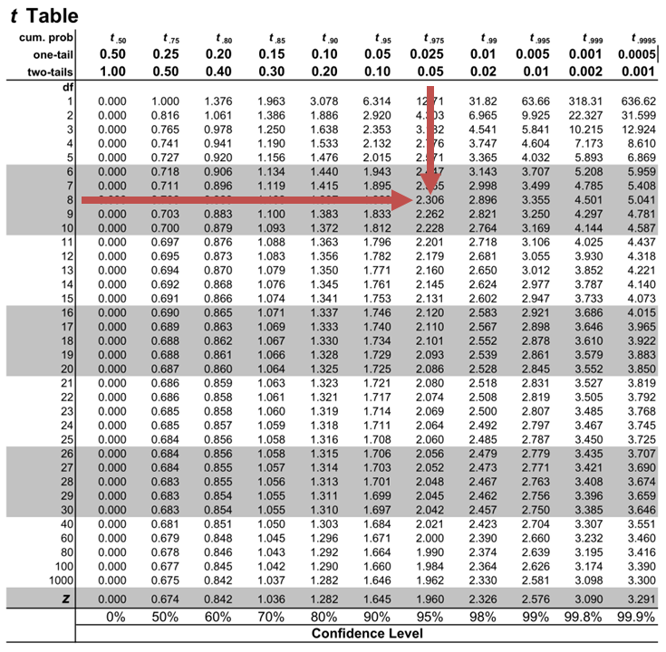
Notice that $|t|>t_{c}$ i.e., ($10.85>2.306$)

Therefore, we reject the null hypothesis and conclude that the estimated slope coefficient is statistically different from one.

Note that we used the confidence interval approach and arrived at the same conclusion.

Question Neeth Shinu, CFA, is forecasting price elasticity of supply for a certain product. Shinu uses the quantity of the product supplied for the past 5months as the dependent variable and the price per unit of the product as the independent variable. The regression results are shown below. $$\small{\begin{array}{lccccc}\hline \textbf{Regression Statistics} & & & & & \\ \hline \text{Multiple R} & 0.9971 & {}& {}&{}\\ \text{R Square} & 0.9941 & & & \\ \text{Adjusted R Square} & 0.9922 & & & & \\ \text{Standard Error} & 3.6515 & & & \\ \text{Observations} & 5 & & & \\ \hline {}& \textbf{Coefficients} & \textbf{Standard Error} & \textbf{t Stat} & \textbf{P-value}\\ \hline\text{Intercept} & -159 & 10.520 & (15.114) & 0.001\\ \text{Slope} & 0.26 & 0.012 & 22.517 & 0.000\\ \hline\end{array}}$$ Which of the following most likely reports the correct value of the t-statistic for the slope and most accurately evaluates its statistical significance with 95% confidence? A. $t=21.67$; slope is significantly different from zero. B. $t= 3.18$; slope is significantly different from zero. C. $t=22.57$; slope is not significantly different from zero. Solution The correct answer is A . The t-statistic is calculated using the formula: $$\text{t}=\frac{\widehat{b_{1}}-b_1}{\widehat{S_{b_{1}}}}$$ Where: $b_{1}$ = True slope coefficient $\widehat{b_{1}}$ = Point estimator for $b_{1}$ $\widehat{S_{b_{1}}}$ = Standard error of the regression coefficient $$\begin{align*}\text{t}&=\frac{0.26-0}{0.012}\\&=21.67\end{align*}$$ The critical two-tail t-values from the t-table with $n-2 = 3$ degrees of freedom are: $$t_{c}=±3.18$$ Notice that $|t|>t_{c}$ (i.e $21.67>3.18$). Therefore, the null hypothesis can be rejected. Further, we can conclude that the estimated slope coefficient is statistically different from zero.

Offered by AnalystPrep